Based on environmental observations collected in a Cambridge attic, can we predict the number of bikers outside?
Introduction
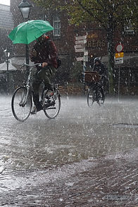
Our work with the rain dataset proved that our sensors can capture rich enough data to infer the weather from ambient conditions indoors. Now we are ready to tackle a more difficult question: can we also predict the number of bikers on the road? The connection is more abstract, but intuition says we should be able to reach some productive conclusions. For instance, if light correlates with time of day, or pressure with rain (as we know it does), then we may be able to infer whether it is prime commuting time. Unlike rain, biker counts are also affected by human factors, such as individual schedules, holidays, events, and road closures. But if that is part of the challenge, it is also part of the opportunity.
Steps
01. Data cleaning
We started our analysis by getting the bicycle traffic data. Cambridge maintains a publicly available dataset of bike traffic past a Kendall Square sensor. The full dataset can be found here. We did not observe any concerning data anomalies.
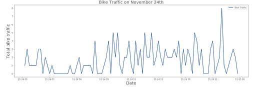
To address timestamps, we saw that bike data is observed every 15 minutes. We began by plotting the bike traffic data. You can also see a zoomed-in graph of the data over the course of one day. The graph reflects the number of bikes passing the totem over a given period of time. We coordinated the timestamps to align with our sensor data.

02. Basic visualizations

Next, we plotted the bike traffic data against the attic sensor data from earlier. We can see that part of the bike data was not collected from index 319 to 380. After investigating more in the data, we learned that the sensor in Kendall square was not capturing data for this time period. Moving forward, we are going to drop this section of data and reindex.
03. Predicting the number of bikers with an OLS model
We began with a basic Linear Regression. We split the data into a 75-25 train-test split, and fit a model to the data. Our accuracy was terrible, with a train accuracy of .14 and a negative test accuracy.
To try to see why that might be the case, our next step was to create a scatter matrix of the different features. The scatter matrix showed a distinct relationship between humidity and pressure, which was unsurprising given weather patterns. We were slightly concerned at this point that we would run into colinearity problems, but at this point we just noted the issue and moved on with our analysis.


Initial results
Next, we tried a multiple linear regression model. It was a slight improvement over the previous model, with an of .13 on the train data and -.01 on the test data.
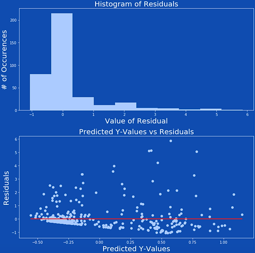
After that, our next step was to look at the residuals. The histogram of the residuals showed that our residuals were not normally distributed, which meant that a linear model probably was not appropriate for this data set. The Y-hat vs Residual plot showed that the residuals were not randomly distributed across the zero-line. This meant that our data does not have constant variance. This makes sense because of the sequential nature of the data.
Our third step was to try polynomial terms. Using degree = 2, we got train accuracy of 0.39 and test accuracy of 0.08, which was a great improvement. With degree = 3, we got even higher training accuracy, 0.51, but much lower test accuracy of -0.03, suggesting overfitting.
We decided that it was time to take a different regression approach.

Polynomial Features model with degree 2
Polynomial Features model with degree 3
04. Can we predict the number of bikers on the road with different regression models?
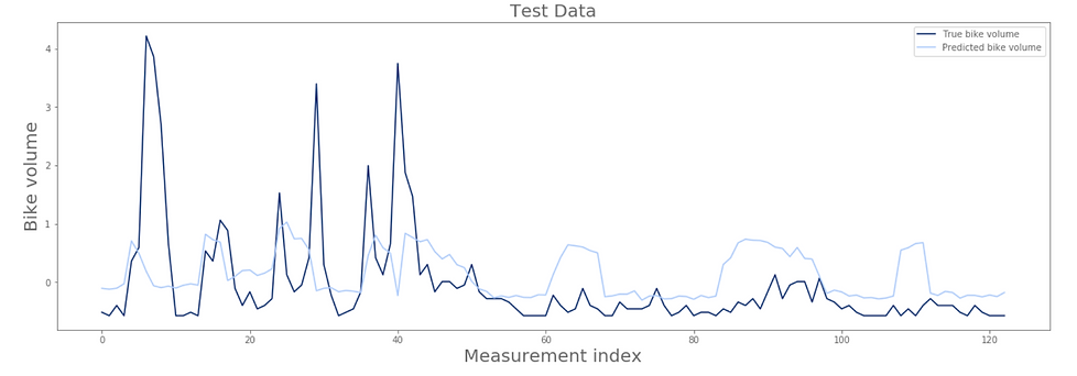
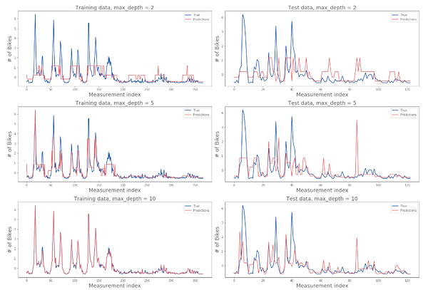
We decided to try a Decision Tree model next. We created models with depths of 2, 5, 10, 11, 12, and 13, and ran each with the training and test data. Below, you can see how our models performed on each set. We got to very good accuracy with the training data, but the test data didn't go above 0.26.
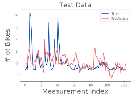
Next, we tried a K Nearest Neighbors regressor using neighbor values of 1 through 10. K=2 appeared to have the best results on the test set, with an R-squared value of 0.43. It still wasn't great, but it was certainly better than the negative accuracy we were getting on the basic regressor.


05. Bring out the big guns
How can we improve this?
As everyone knows, AI is magic and any sufficiently nonlinear ML technique is AI, so we tried brute-forcing a number of neural net approaches.
Our initial model showed overfitting, so we tried again with two dropout layers. It was slightly better, but not much, so we added in a layer of batch normalization. Finally, we tried higher-order features, but all of this only made the overfitting worse.

Going back to the data
After adding KNN, dropout, normalization, and augmentation, we returned to the data to try to eke out some final performance improvement. This isn't Amsterdam - bikes are mostly a commuter thing, and thus principally in use during weekdays. The weather doesn't tell us whether it's Saturday, so intuitively it seemed likely that we would never be that great with sensor data alone. We decided to power up and add the day of the week. We had to reprocess the data to get the weekday, but that was a sacrifice that Python was willing to make. We also added in some regularization to try to compensate for overfitting.


Unregularized

Regularized
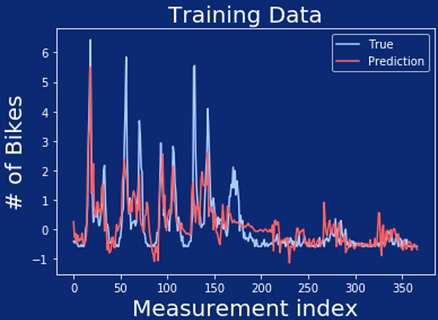
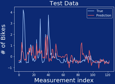
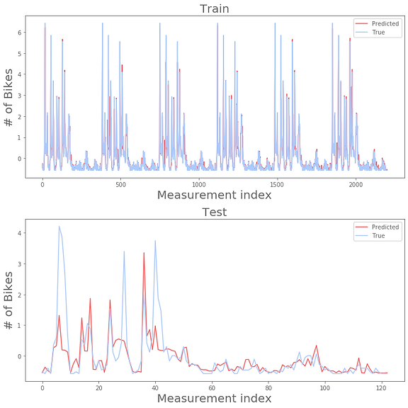
In the end
R-squared train: 0.94
R-squared test: 0.51
A very slight improvement from adding the day of the week! Not bad for a couple sensors in a Cambridge attic.